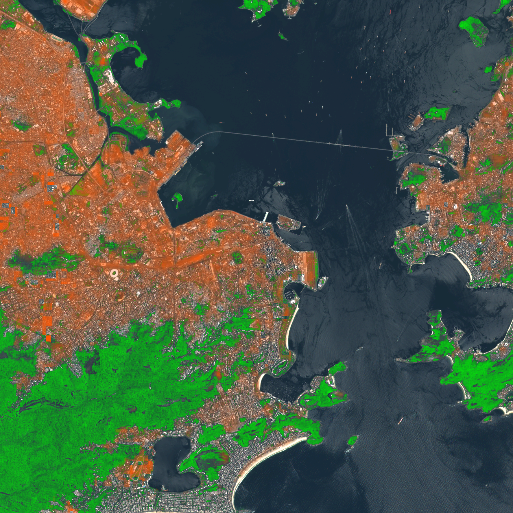
Urban Heat & Vegetation Analysis
Evaluating the relationship between heat indexes and vegetation indexes in urban environments
July 8th, 2026
Preface
It is well documented that proper placement of urban vegetation has a strong impact on localized temperature levels. Individual streets with overhead vegetation have been found to hold significantly lower ambient temperatures when compared to neighboring streets without vegetation. While this relationship has been well established by empirical measurements, this report attempts to review several attempts to model the same pattern using satellite remote sensing data.
Data Collection
One of the key challenges this report attempts to overcome is that neither local ambient air temperature nor vegetation metrics can be measured to the same empirical quality from 800 kilometers above the Earth’s surface. Instead, we must decide on proxy metrics that we will call the Thermal Index and Vegetation Indexes respectively.
While collecting data for these metrics, three basic constraints were considered:
Vegetation and Thermal indices must represent the same area at the same scale/resolution
Thermal indices must be collected during the hotter months of the respective region
Vegetation indices must me collected within 2-3 months of the thermal index to ensure vegetation currency
With these constraints in mind, this report used the following methods to collect Thermal and Vegetation Indexes.
Thermal Index
Land Surface Temperature (LST) was used as the base thermal index for this report. Microsoft’s Planetary Computer was used to extract LST data from Landsat 8/9 using Collection 2, Level 2. Specifically, given a particular AOI, the “ST_B10” asset was considered to extract LST. This asset uses Landsat Band 11 data which measures Long Wave Infrared (LWIR) Radiation (10.9 micron wavelength) and automatically accounts for atmospheric interference to estimate a surface temperature in Kelvin. This temperature is then adapted to Celsius values for ease of review.
It is important to note that LST itself does not measure the ambient air temperature of a given region, however, it has become an industry to measure a given land area’s capacity to retain heat. LST is estimated by measuring LWIR at the top of the atmosphere and transforming it to account for atmospheric disturbances. This method results in a highly accurate estimate of the LWIR emitted from the Earth’s surface which can then be easily converted to a temperature reading using the Stefan-Boltzmann method. It is important to comment on this end-to-end process because it requires an accurate look up table managed by the US Geological Survey (USGS) which is not complete for the entire Earth’s surface. This incompleteness creates “No-Data” pixels where LST cannot be accurately estimated. This was accounted for by using a filter to reject scenes with too many “No-Data” pixels.
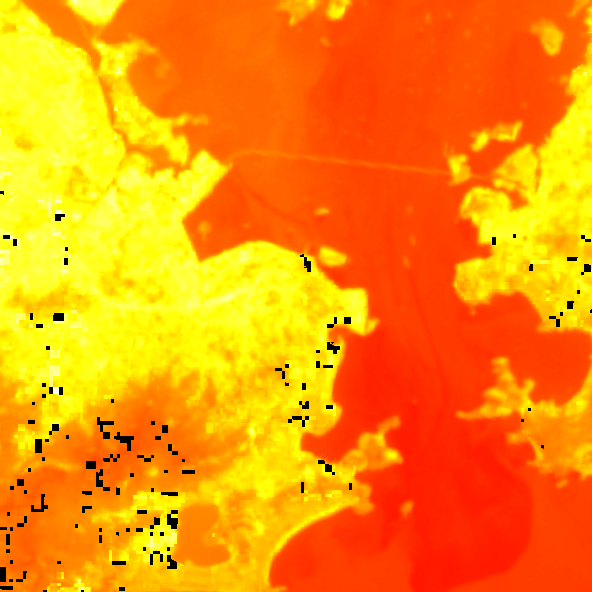
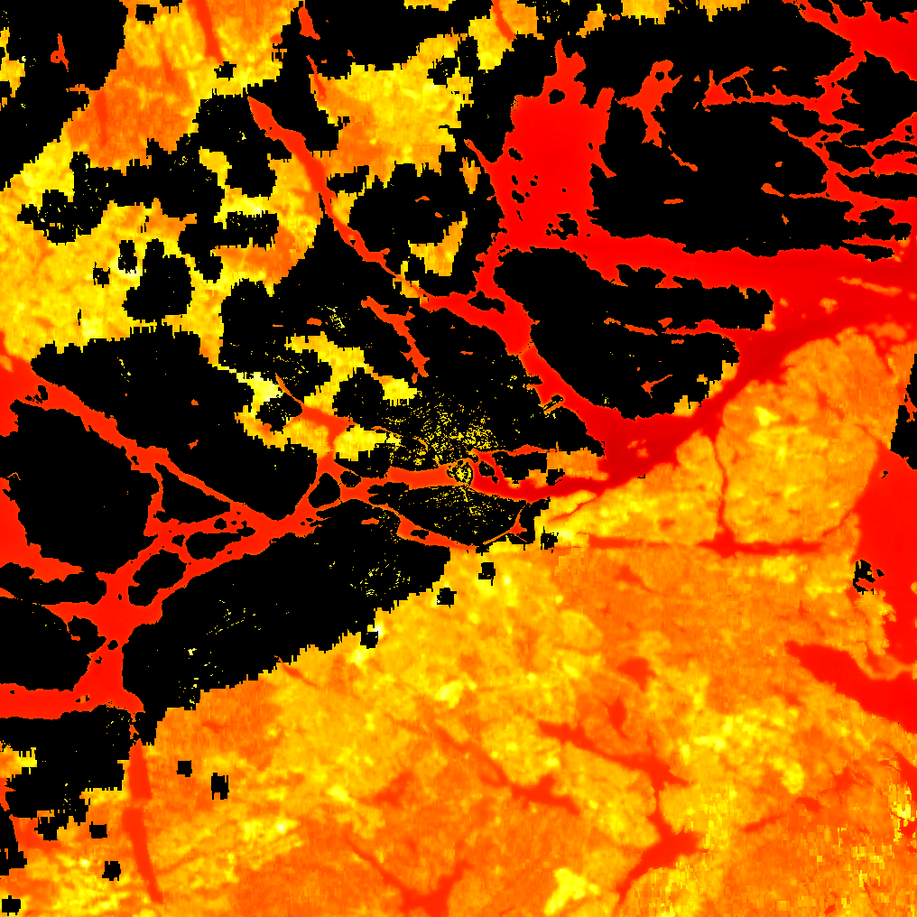
The result of this collection process as a geo-referenced xarray of pixel data where each pixel represents the thermal index of a 30m x 30m square. Below is a sample of this type of image. Note the missing black pixels reprenting "No-Data" areas where LST could not be reverse calculated from top-of-atmosphere observations.
Vegetation Index
Many different methods have been used to measure the vegetation content in a given area from satellite data. Several of these were detailed below, but all rely on a subset of red and infra-red data. This data was also extracted from Planetary Computer using the Sentinel2 Collection 2, level 2a historical data. Specifically, bands 4 (Red), 8 (NIR) and 11 (SWIR) were used. These bands are specifically helpful in measuring vegetation content because of the contrast in these bands between vegetation and other landmass types. These bands were then transformed into the following indexes.
Normalized Difference Vegetation Index (NDVI)
By far the most popular vegetation index, NDVI is calculated by dividing the difference between the red and NIR bands by their sum. This is method takes advantage of the fact that chlorophyl in healthy plants absorbs red light while reflecting NIR radiation at a rate that is different from most other landscapes. The difference helps to highligh vegetated areas from their surroundings.
Soil Adjusted Vegetation Index (SAVI)
SAVI is very similar to NDVI but accounts for sparsely vegetated areas by adding a scalar value L to both the denominator of the Index and as a multiplicative factor of (1+L). This adjustment to the index creates more contrast for areas with vegetation when compared against areas of no vegetation.
Normalized Difference Moisture Index (NDMI)
NDMI does not focus on whether a given pixel contains vegetation, instead it attempts to measure the health of vegetation if it is present. It does this by measuring the presence of moisture by dividing the difference in the SWIR and NIR bands by their sum.
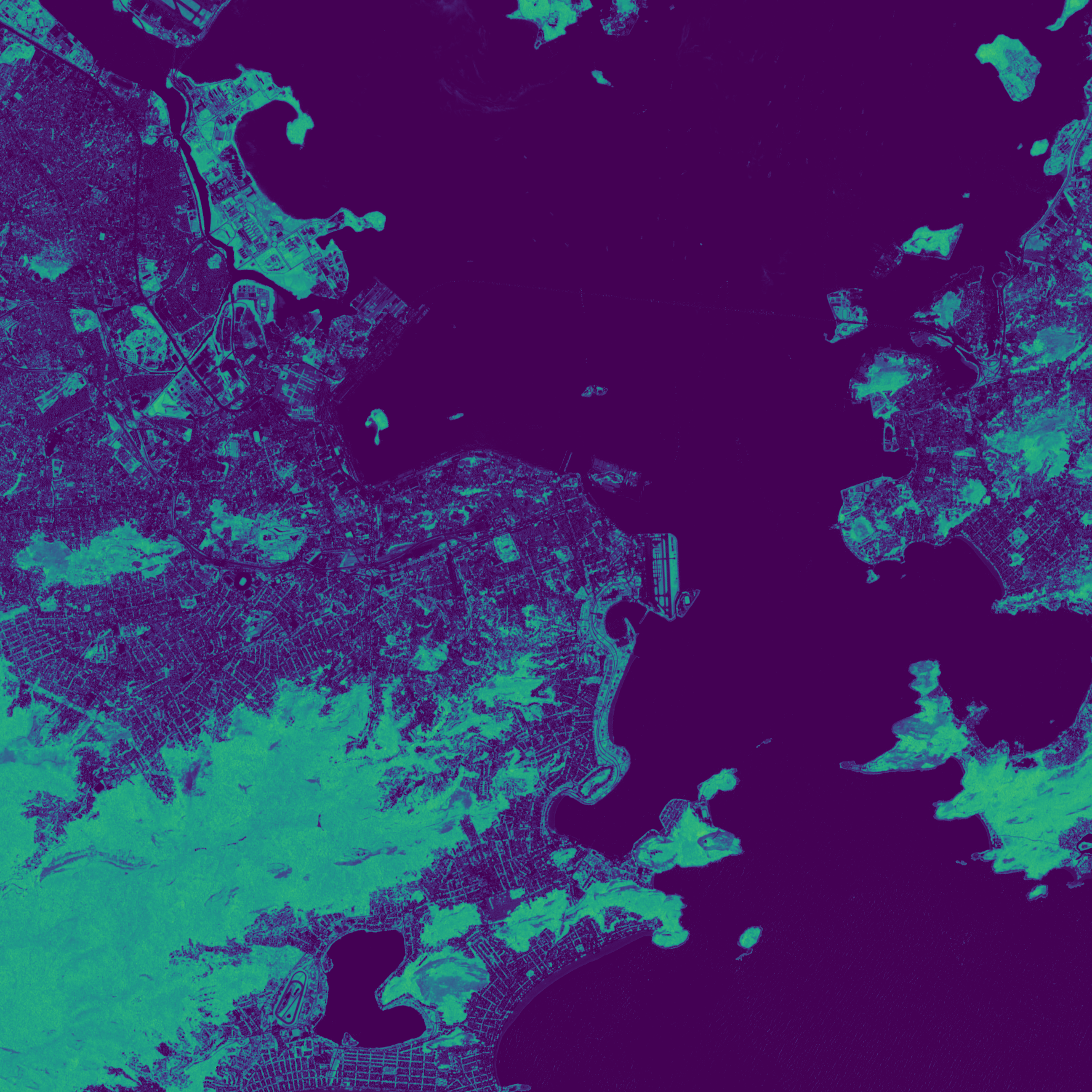
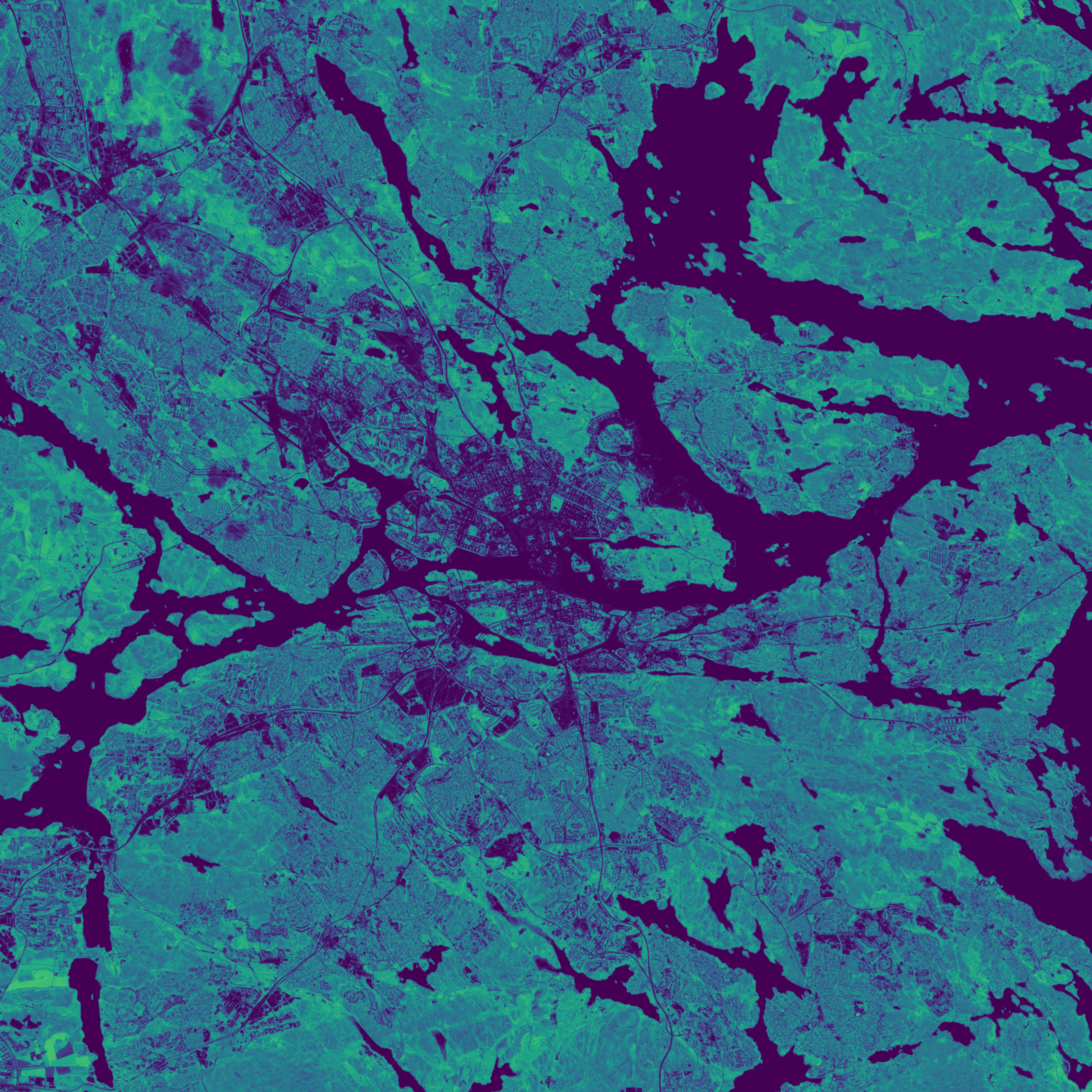
For visualization purposes, below is an image of the NDVI for Rio de Janeiro taken on November 18th, 2024, three months before the LST index shown above. Note how city streets in some parts of the city are more visible than others.
Data Collection
The data for the indexes defined above were collected using the “combined_observation” class in the linked GitHub repository. This class receives a target point (often the centroid of a target city) and an area of coverage (in square kilometers) and performs the following process:
• Defines the Area of Interest (AOI)
• Recursively attempts to collect Sentinel2 and Landsat Stac Items to cover the AOI meeting the following requirements
• Observation during the warm season for the AOI’s area of Earth
• Temporal consistency between Landsat and Sentinel
• A low enough fraction of cloud cover (which slowly increases if a lower threshold cannot be met)
• A high enough percentage of coverage (for Sentinel data this is 99.9%) with meaningful data
• Down selection to only the most useful Stac Items
• Once Items are collected, LST, NDVI, SAVI, and NDMI are calculated
This process was performed for a list of 32 cities with representation from all of the Earth’s warm climate zones for both 750 square kilometer and 300 square kilometer zones. The 750 sqkm assessment resulted in 15 qualified city scenes and the 300 sqkm assessment resulted in 21 qualified scenes.
Finally, a set of 234 city observations at 250 sqkm scale was collected for broader data collection.
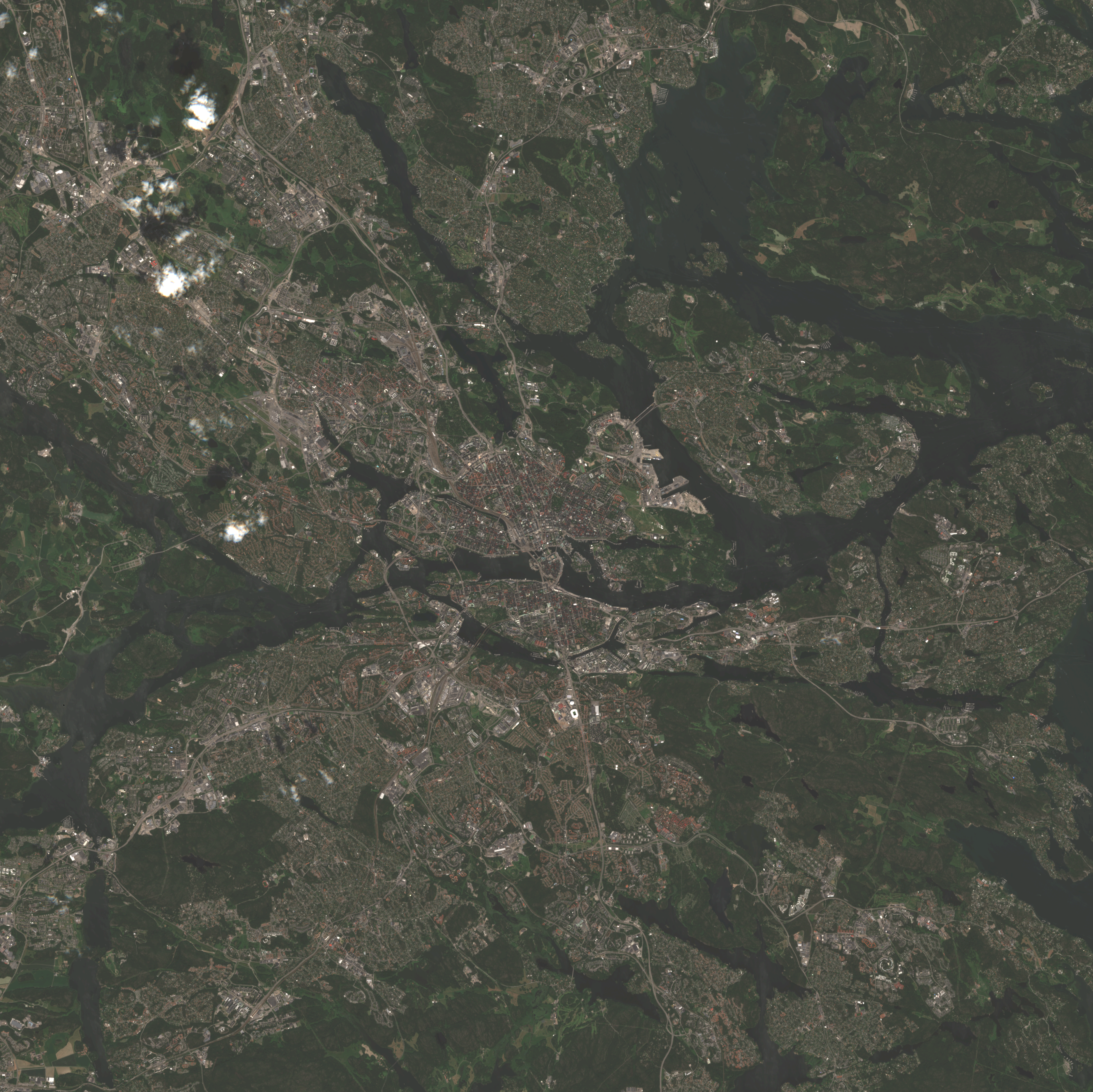
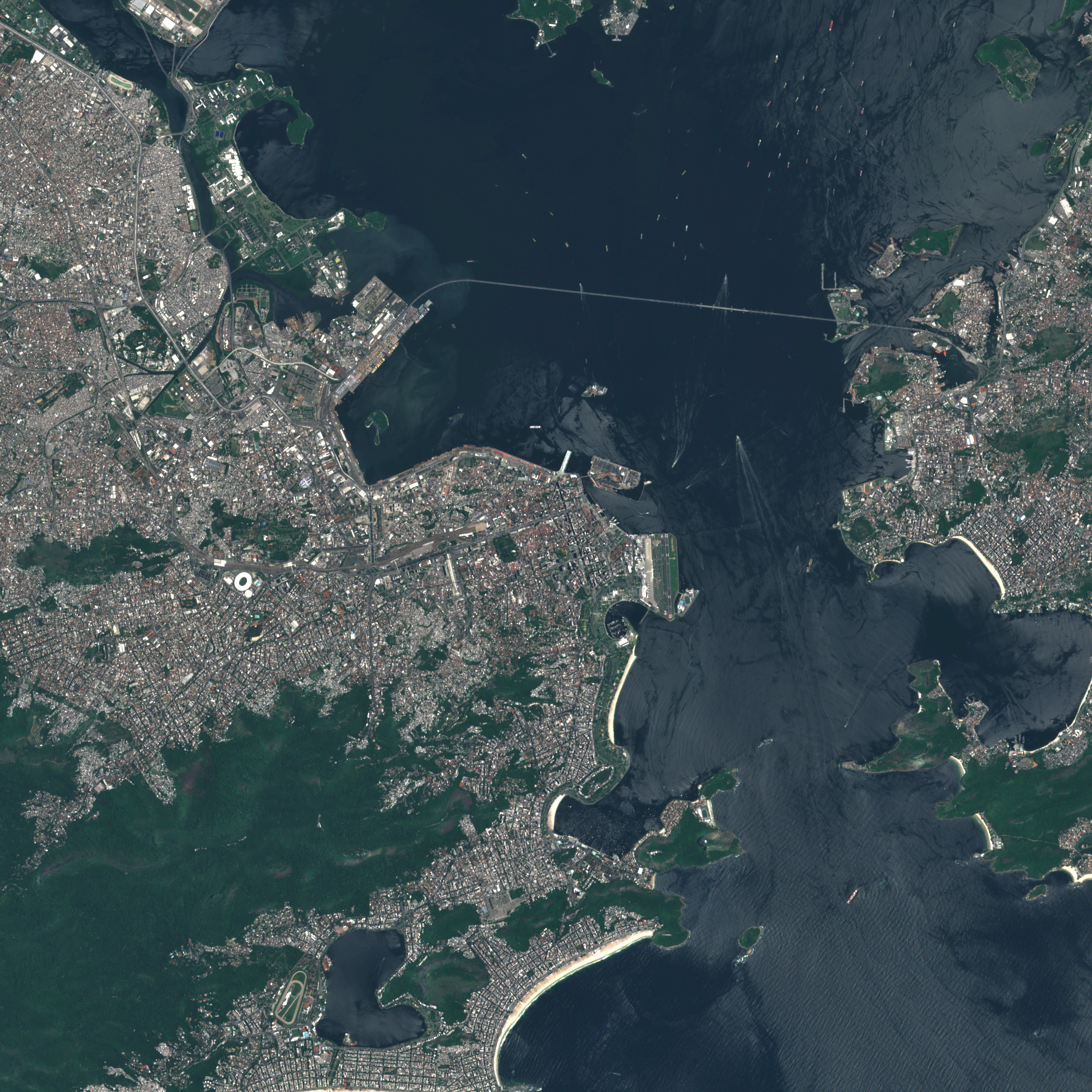
Below are examples of a 750 sqkm scene taken of Stockholm and a 300 sqkm scene taken of Rio de Janeiro.
Methods
With the data collected, several approaches were taken to compare the various vegetation indexes against the thermal index. The first step of each of the methods below was to down sample the higher resolution vegetation indexes such that the geographic representations of each pixel aligned across LST and Vegetation Indices. A mean resampling approach was taken to this down-sampling such that each new vegetation pixel was the mean value of the original pixels contained within it’s area. When resampling from 10m resolution to 30m resolution, this meant that each resulting pixel was the average of the nine 10m-by-10m areas contained within the 30m-by-30m area.
Each of these evaluation methods were taken for 234 cities across the world at a scale of 250 square kilometers. Results for sample cities and the collective group of 234 cities is presented for each method below.
Pixel-wise Masking with Pearson Correlation & Regression
The first comparison made used a simple pixel-wise approach. This method aligned each pixel in the vegetation index against each pixel in the thermal index. After this alignment, “No-Data” pixels and invalid pixels were removed from each index through a validity mask.
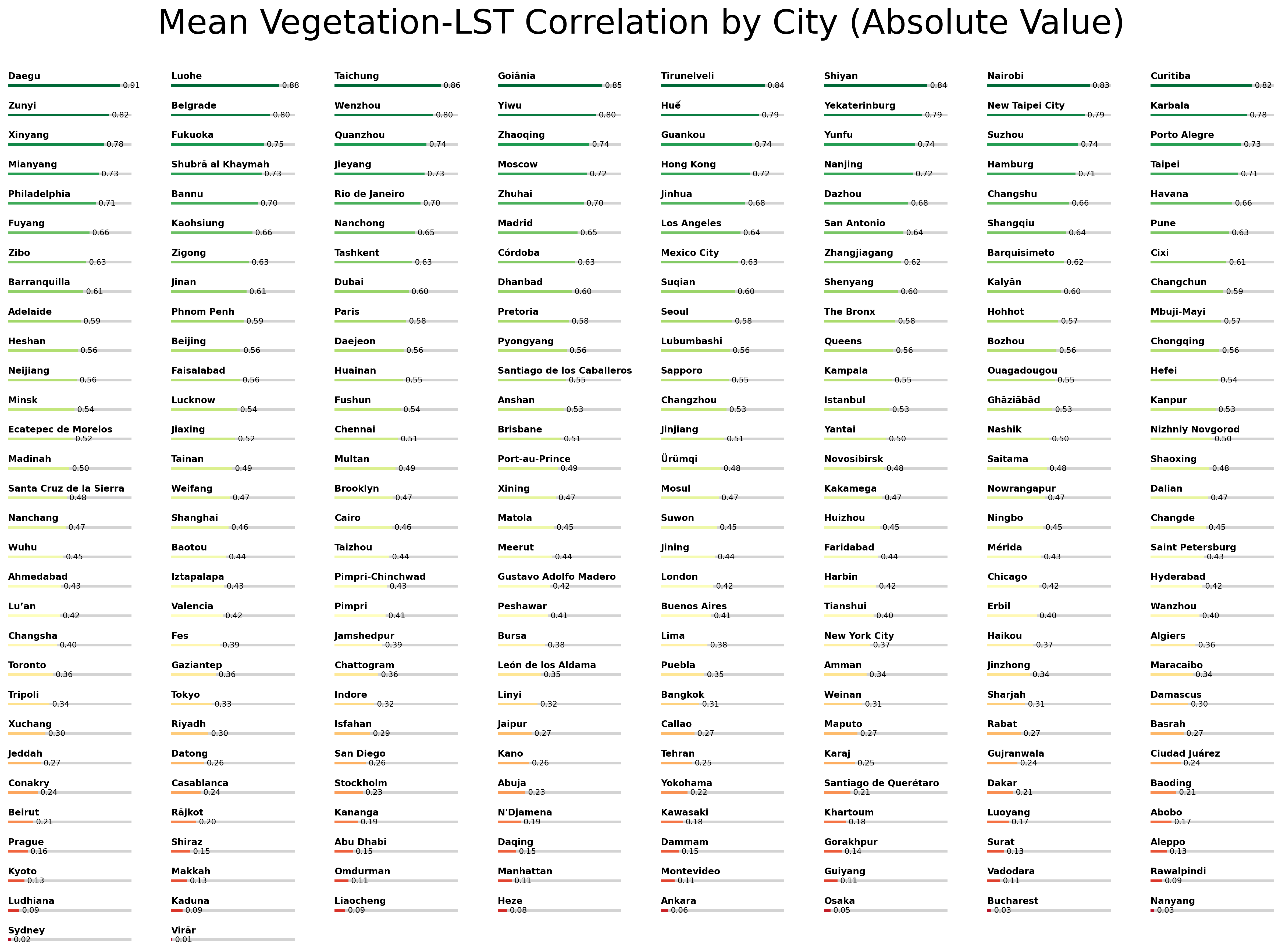
The resulting valid masks were compared for statistical significance using a Pearson Correlation and a regression slope. Pearson Correlations offer a suggestion to the correlation between to datasets such as those constructed here where a value of 1 shows a strong correlation and a value of 0 shows no correlation. Typically, a Pearson correlation between 0.3 and 0.5 suggest moderate correlation between two sets while a value above 0.5 suggests strong correlation. In addition a regression slope measures the direction and “steepness” of the correlation between two datasets. A positive regression slope indicates that two values are positively correlated while a negative slope would suggest a negative correlation (e.g. for vegetation and LST we would expect a negative correlation because if there is more vegetation, we would expect lower temperatures). A sample of this correlation analysis is shown below:
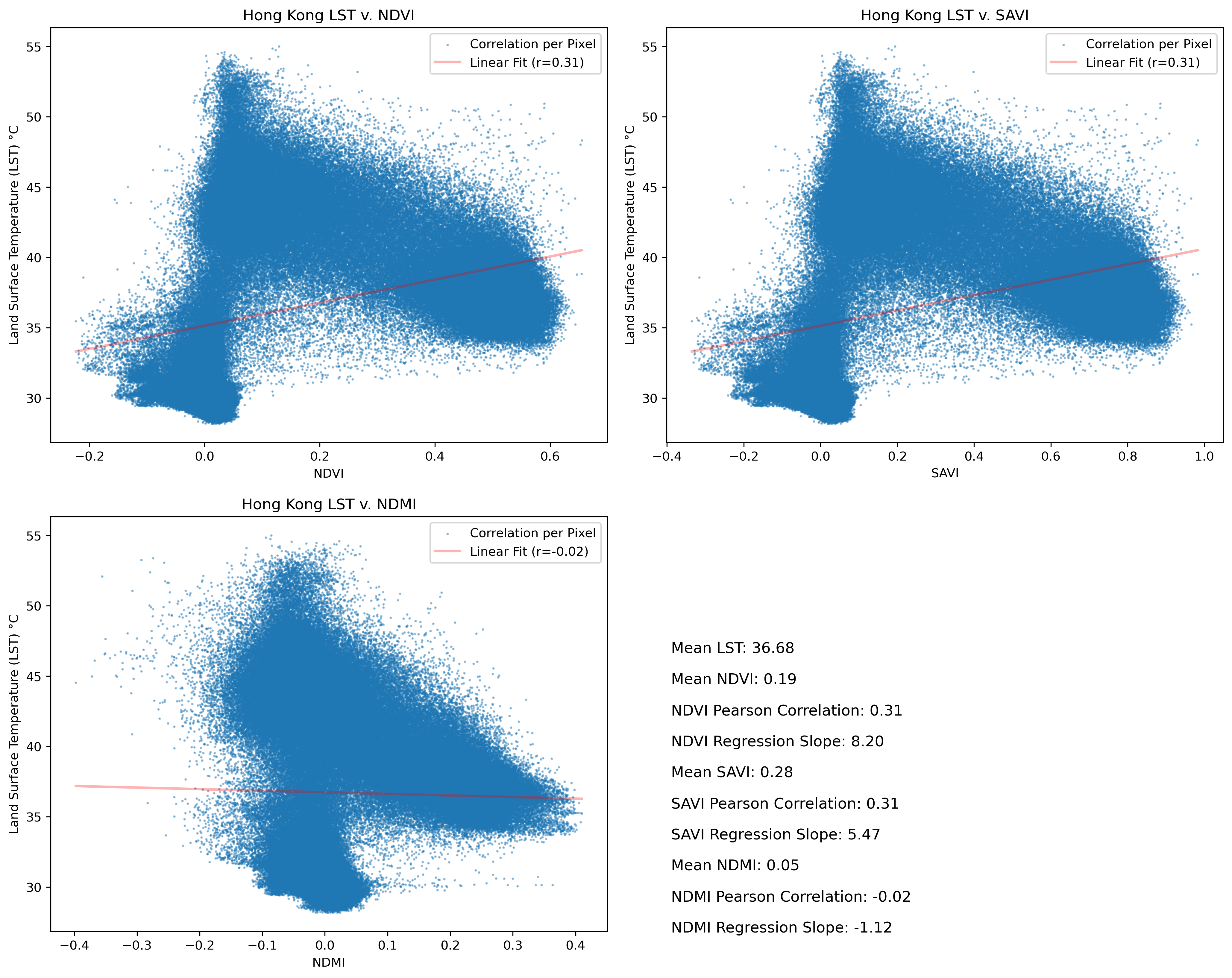
While the correlation is moderate one significant characteristic stands out immediately, the slope of linear regression for each index type is positive indicating a positive correlation. This is unexpected as presence of vegetation should have an inverse relationship to the presence of heat. But after further analysis, it become apparent that this observation (along with most other large cities across the globe) contains a large body of water. Large bodies of water possess the unique characteristic that they are often cool relative to their surrounding land-masses but also score very low on most vegetation indexes. This quality has the potential to significantly skew analysis using the metrics of this study.
Below is a collection of observations of cities where the thermal index inversed such that the coolest areas are shown in light blue. Note between the visible image and the overlay how the overlay fits well over large bodies of water. Since vegetation indices often have very low values over water, it is clear how this data would skew the correlation.
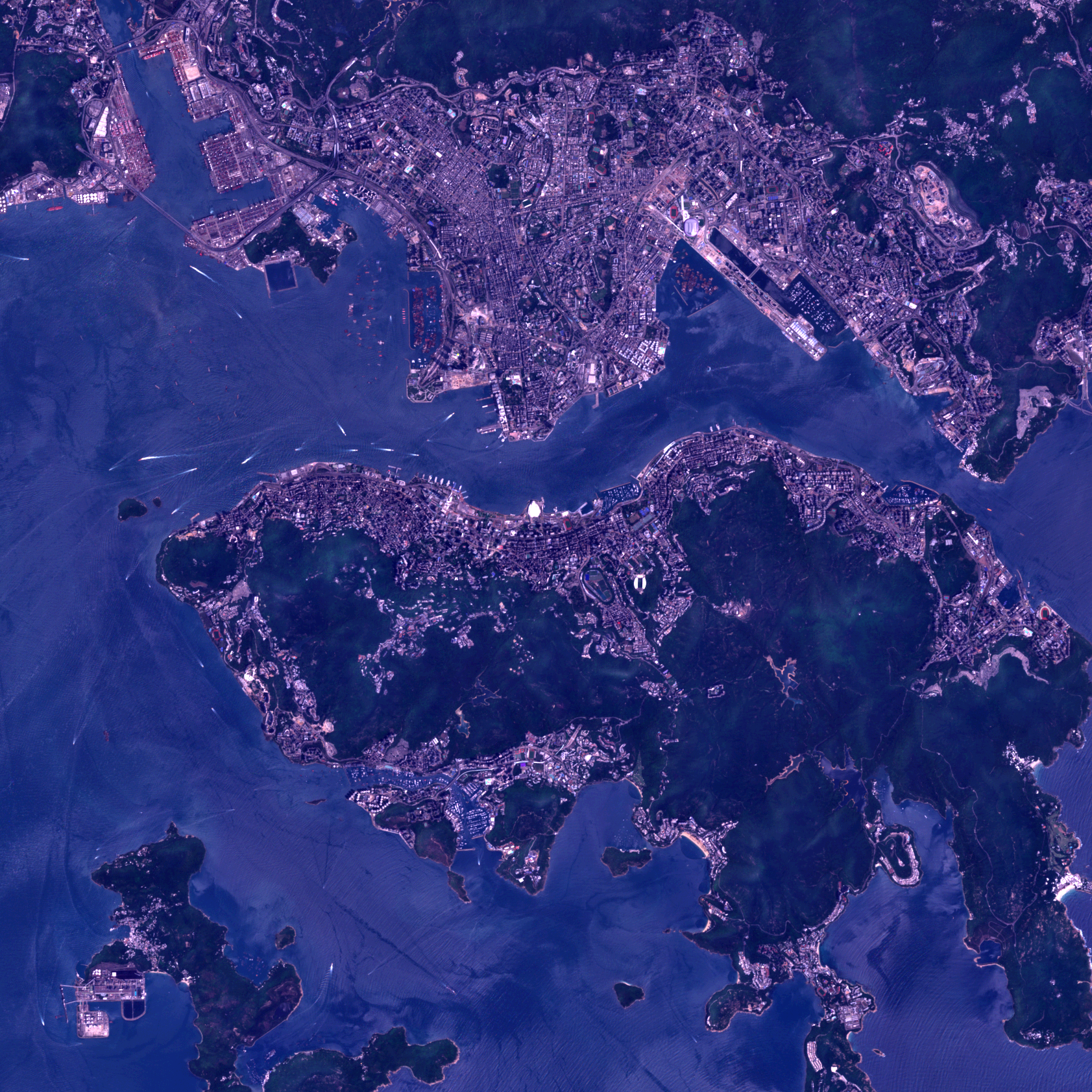
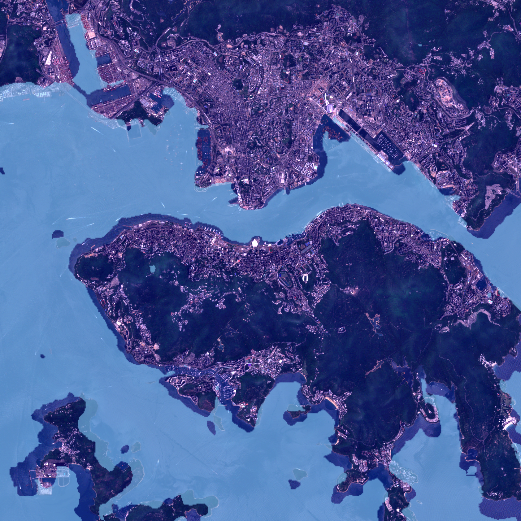
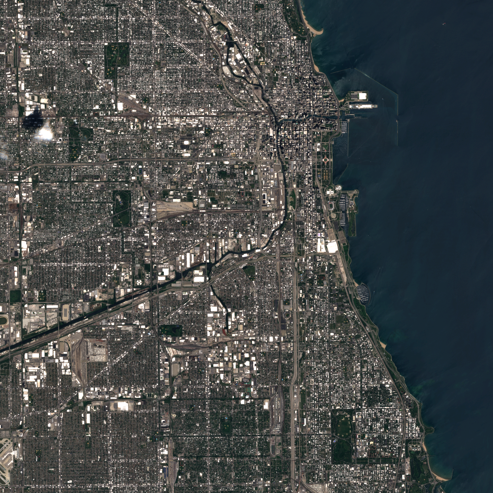
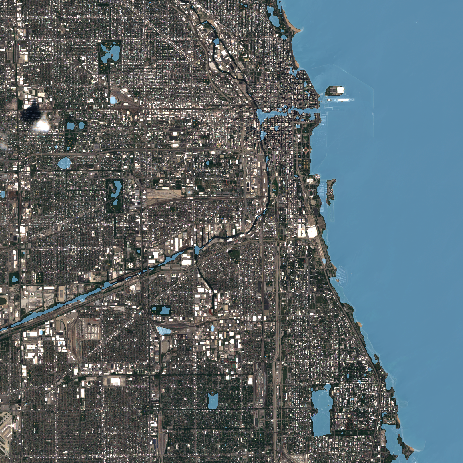
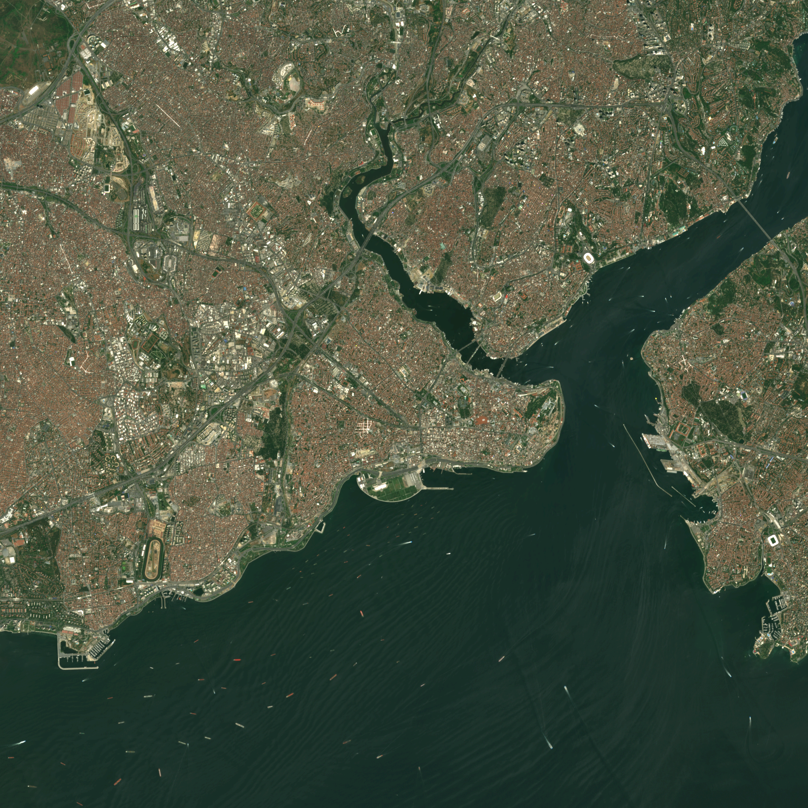
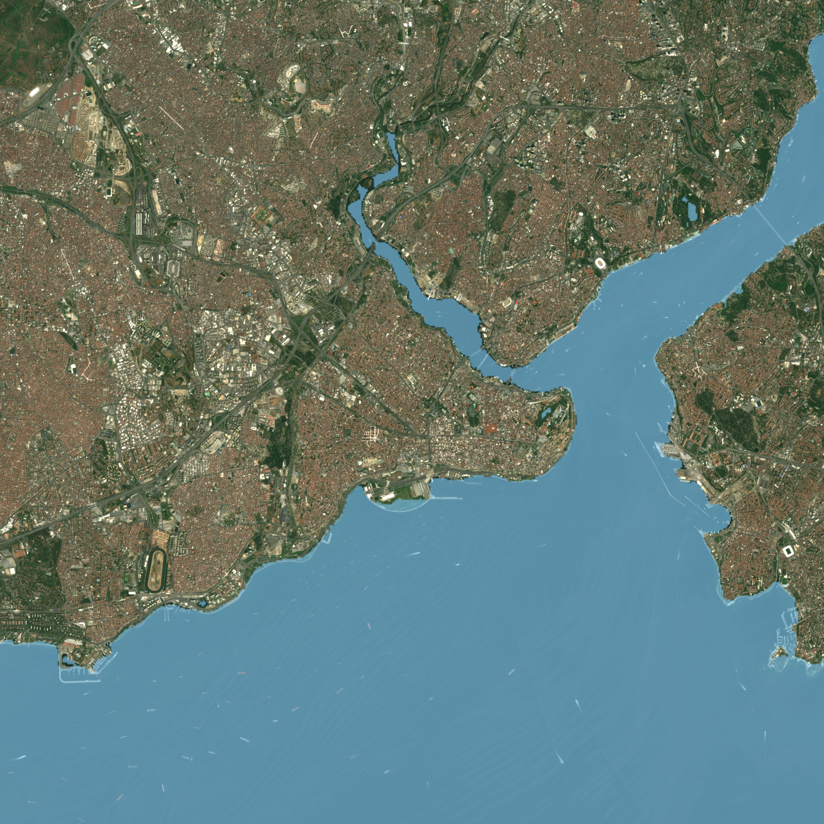
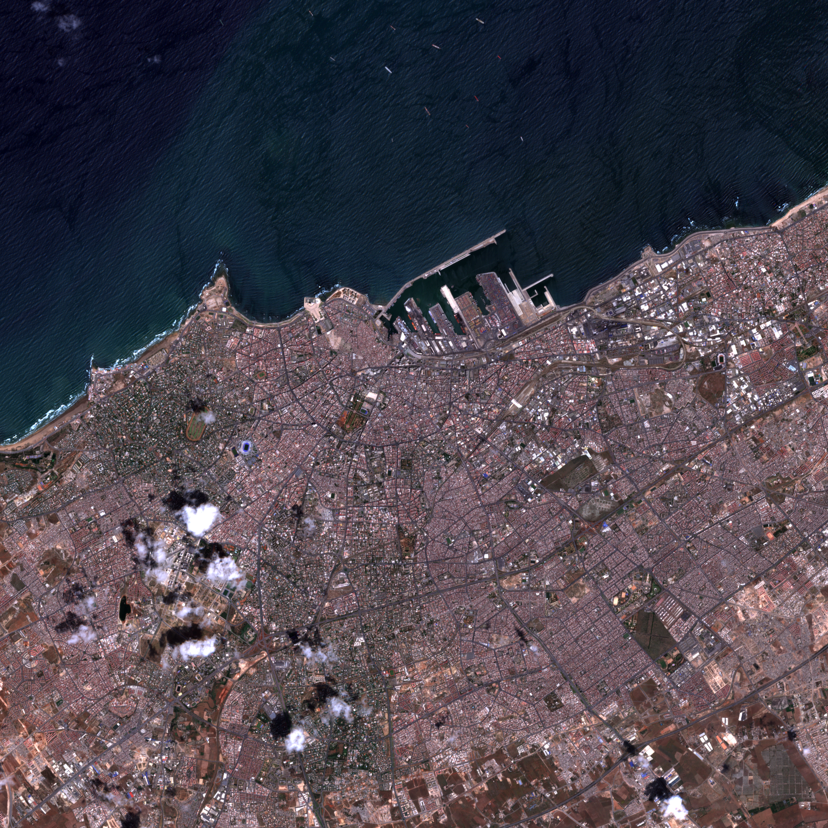
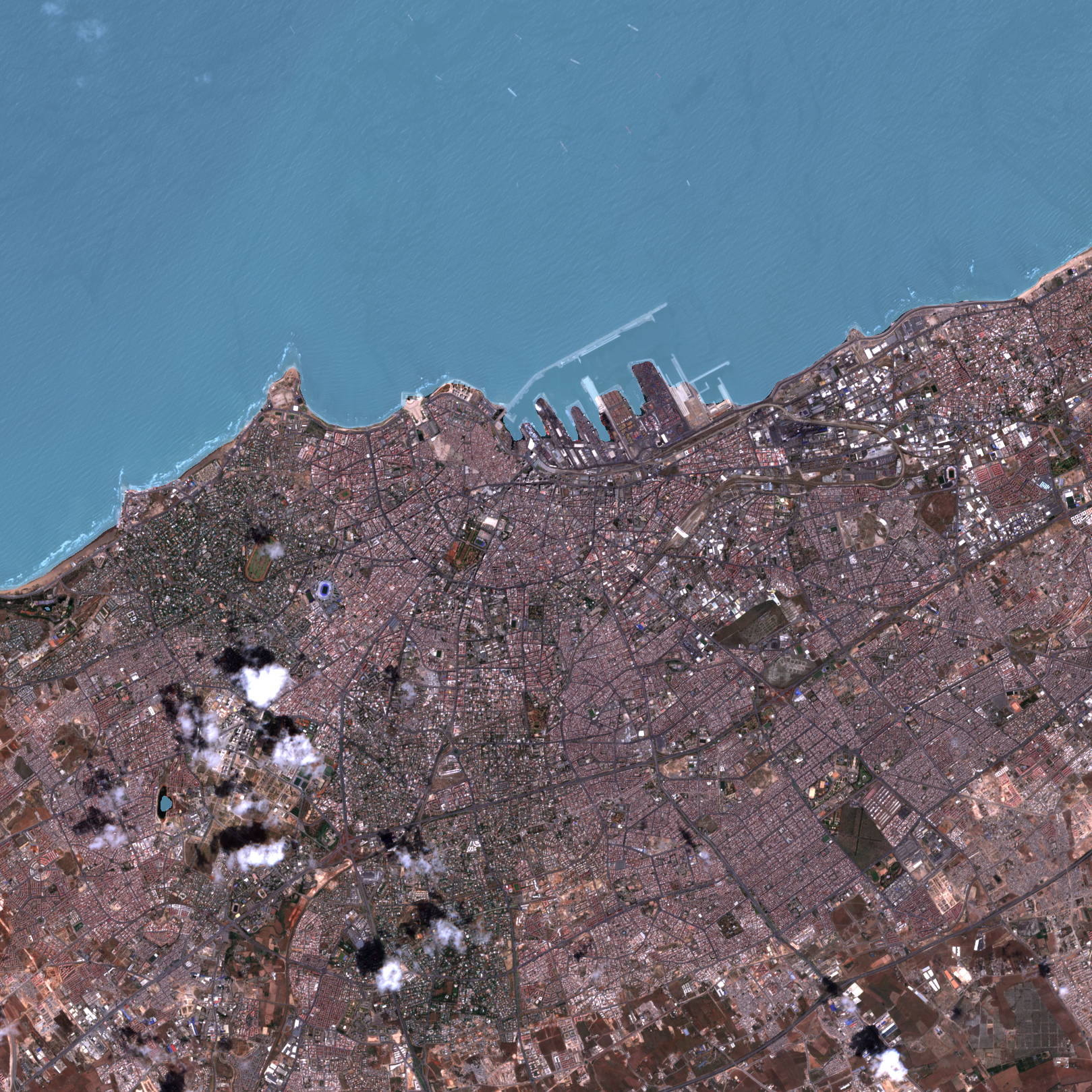
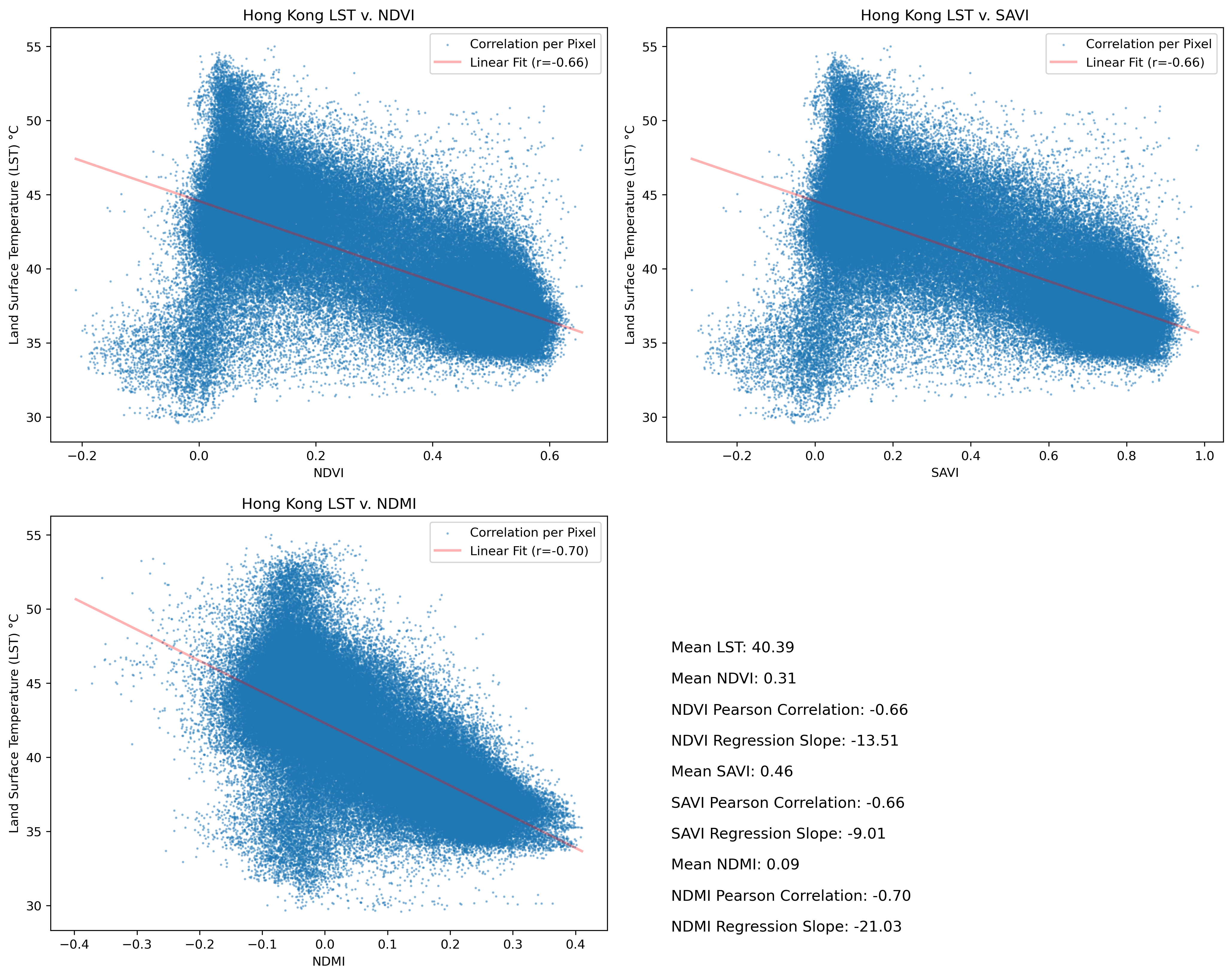
To perform a more accurate analysis of the landmass then, we must filter out of our analysis pixels that are completely water. This was achieved using the Sentinel2 Scene Classification Layer (SCL) asset. This asset allows us to create a similar validity mask for pixels containing water as that used above for “No-Data” pixels. With this mask applied, the scenes were re-evaluated. The results for the same city evaluated above (Hong Kong) are below. Note how with water pixels removed, the slope of the regression line has become negative, suggesting the inverse relationship between vegetation and thermal indices that we were expecting.
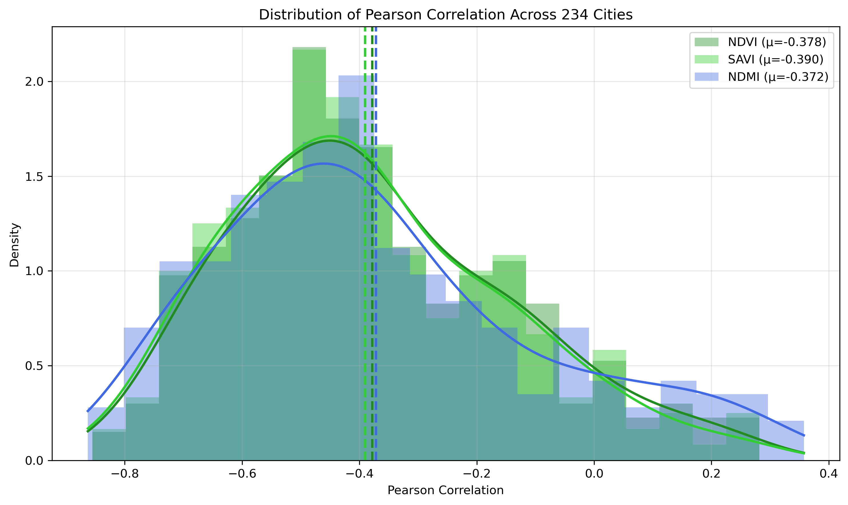
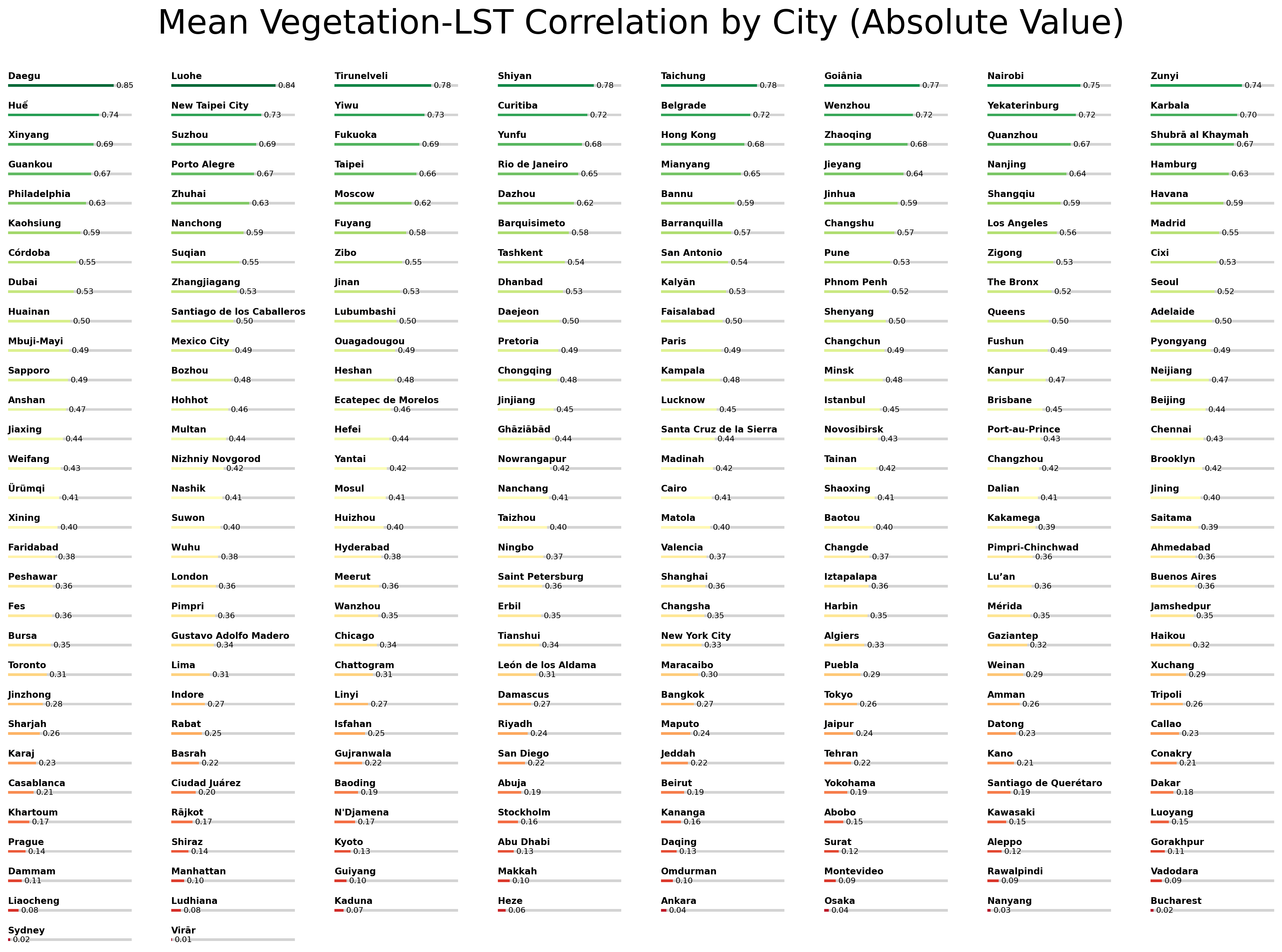
Below you can see a summary of all the results evaluated across 250+ cities across the world for each of the evaluated vegetation indices (NDVI, SAVI and NDMI).
Pixel-wise Localized Mean Masking
Another method of correlation is to abstract the vegetation index pixels based on their local mean. To do this, we keep the same number of pixels as originally produced, but instead of taking each pixel at measured value, each pixel is changed to the average index value for all other pixels within a certain distance of that pixel. In this case, we selected 150m as the averaging radius. This value was chosen in an attempt to keep values relatively localized in a way that would still be meaningful
This method is beneficial because it “smooths” the index values to minimize anomaly pixels for a given LST measurement. This is beneficial because LST varies less quickly over space. This is method should be approached carefully, however, as the averaging can act as an abstraction that could present false correlation.
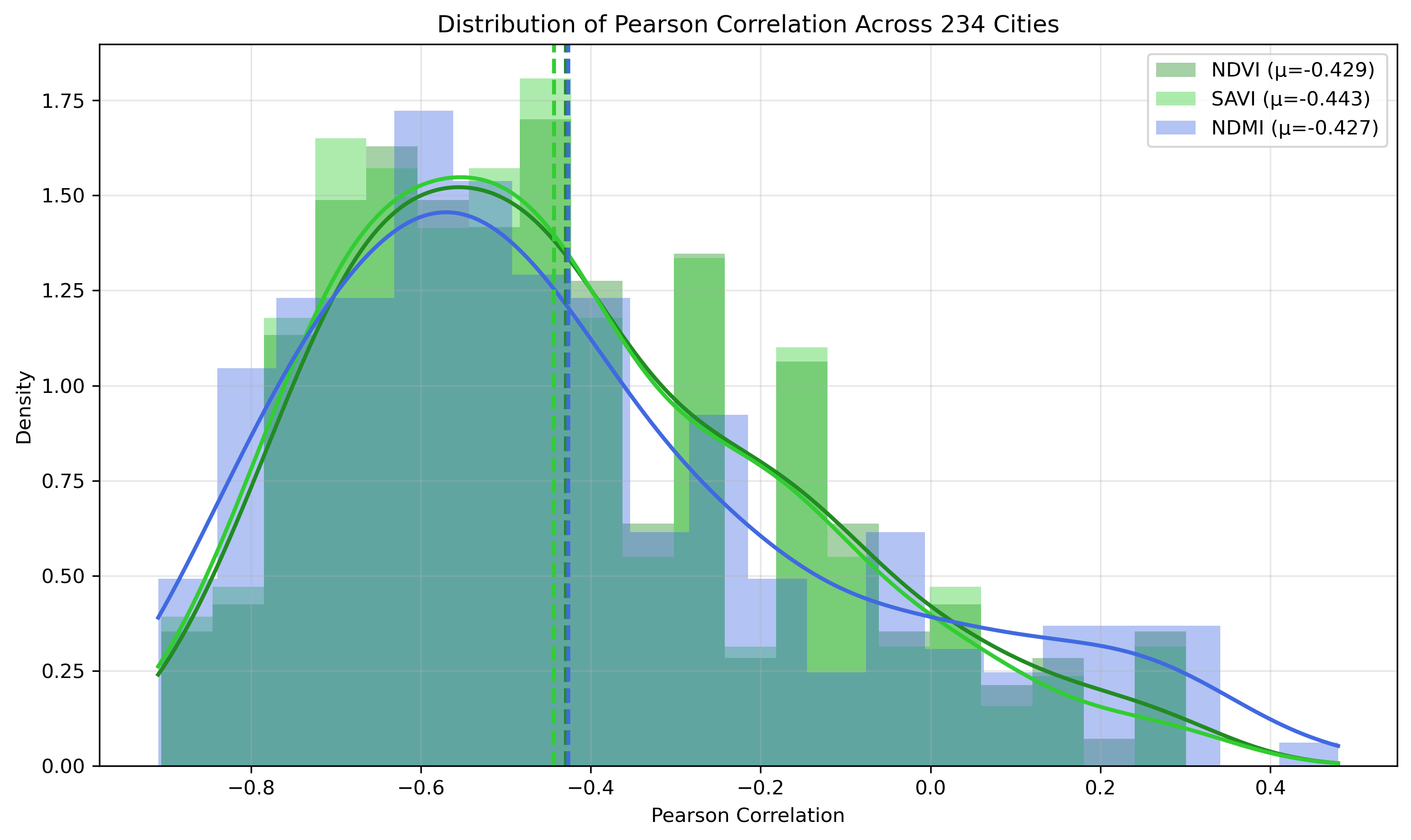
After the index pixels are averaged, the correlation is processed as with the Pixel-wise Masking method. The results for this method can be seen below:
Intersection Over Union (IOU)
The final method of comparison for this report comes from a typical method for scoring segmentation Machine Learning models against ground truth. IOU is a score which compares binary (true/false) values over a scene.
To use this method of comparison, the temperature and vegetation indexes must both be converted to binary values such that the thermal binary mask presents true values where a pixel could be considered a thermal anomaly (i.e. a value that is significantly higher than the scene’s mean temperature); and such that the vegetation mask is true for the pixels where there is confidently no vegetation based on the given index.
To visually demonstrate this relationship, the images below have masks where the Thermal Index (Red) is High enough to be considered an anomoly and the Vegetation Index (Blue) is Low enough to be considered to hav n significant levels of vegetation. Note the locations where the overlay appears purple, these are considered the "Intersection" of the two masks, while the areas that are blue, red or purple are considered the "Union" of the two masks. The IOU score is then the ratio of the Intersection to the Union.
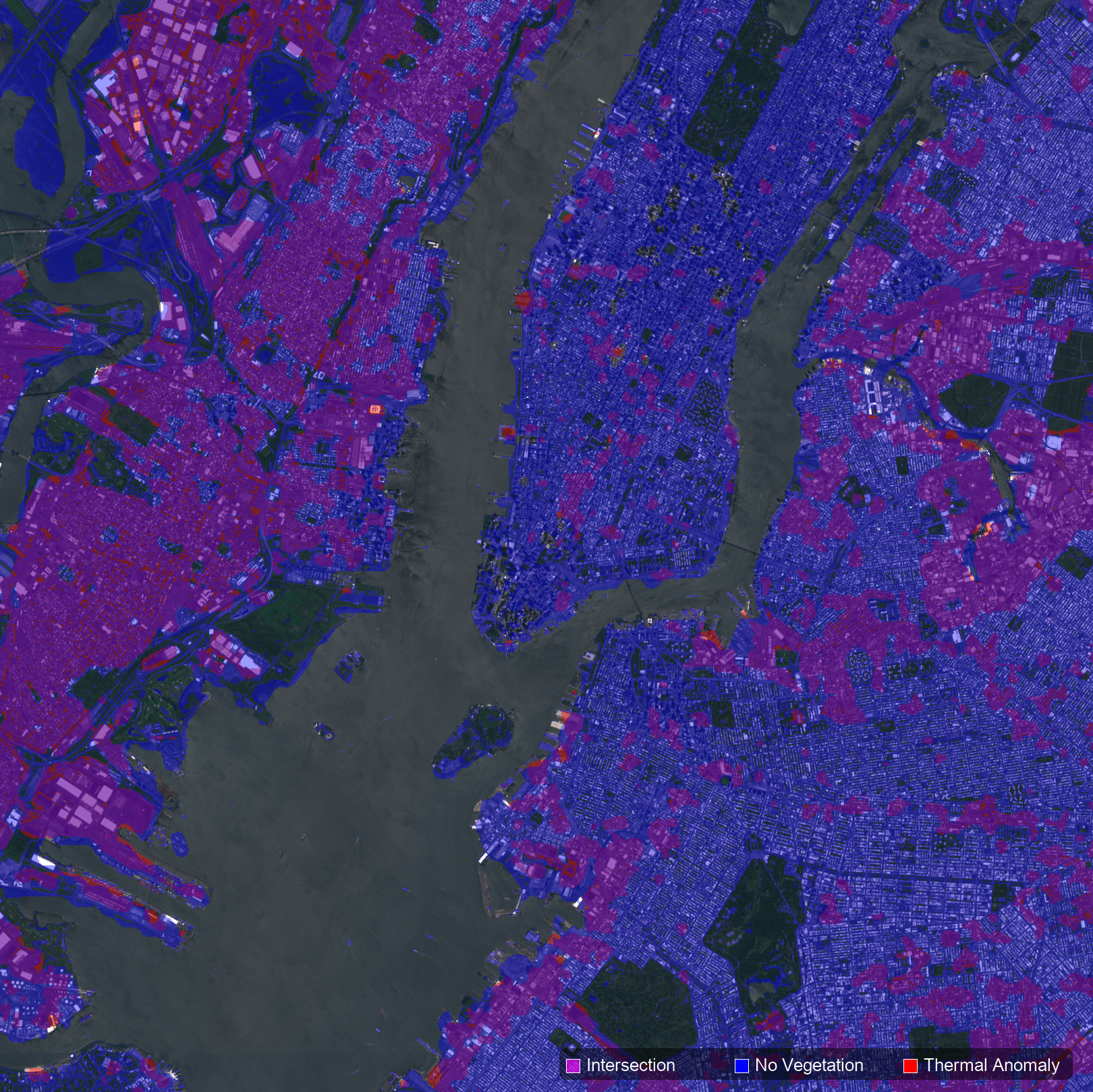
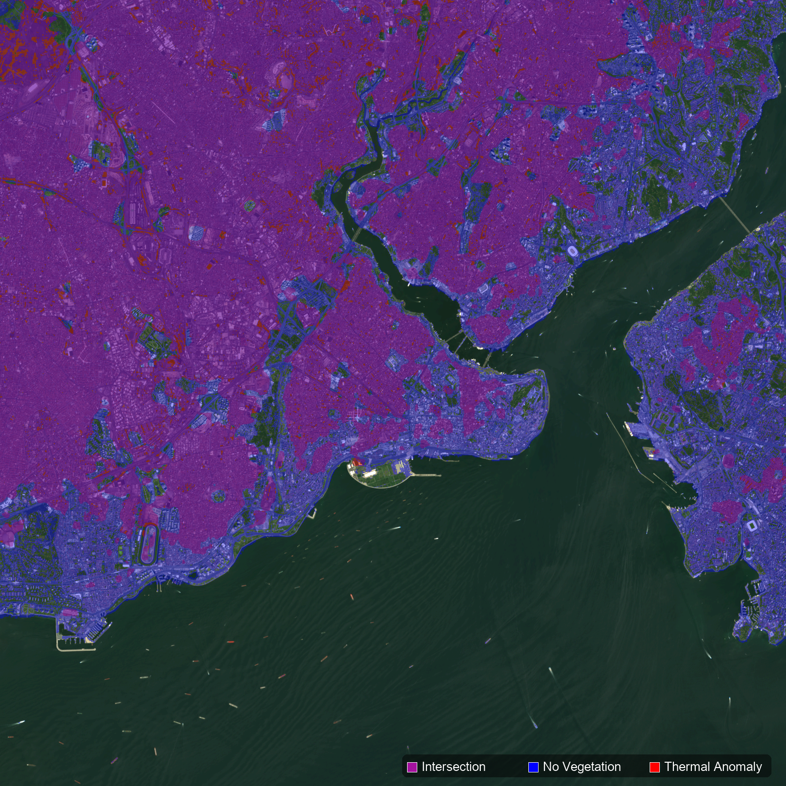
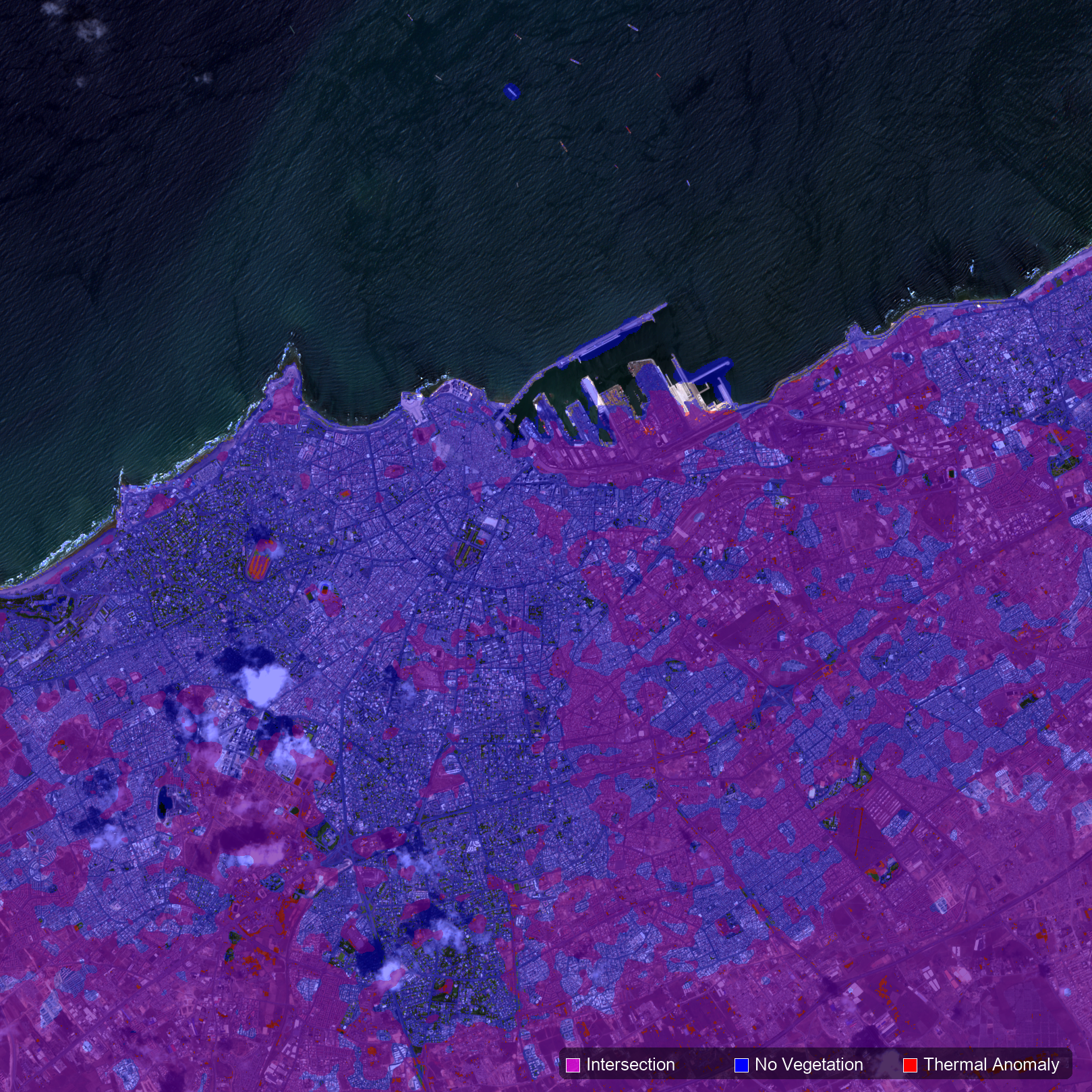
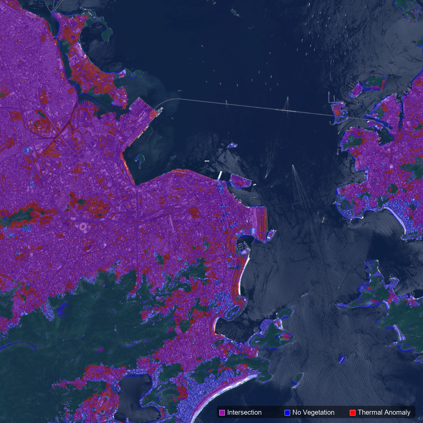
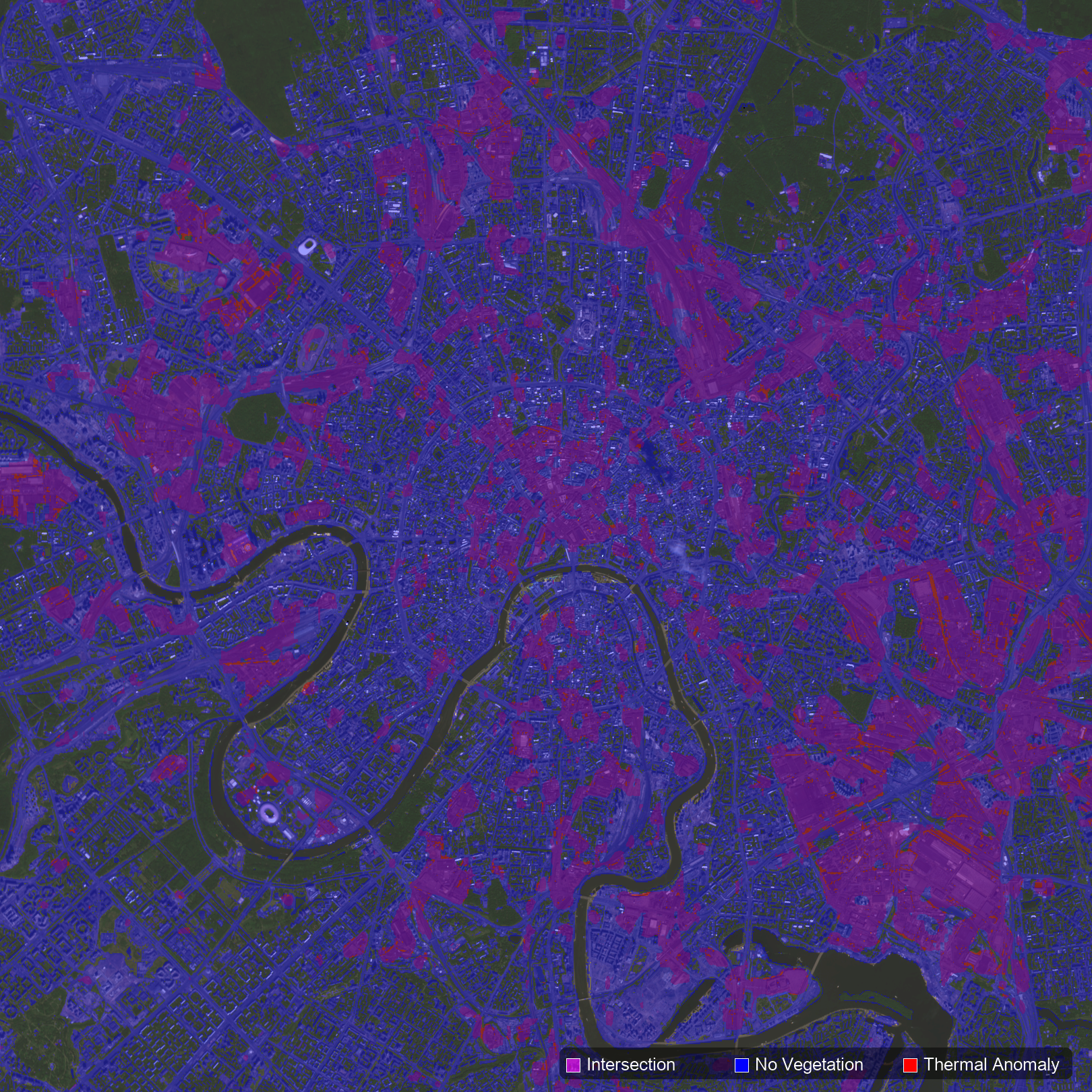
For the thermal anomaly, this masking was achieved by determining the pixel’s deviation from mean (pixel value – scene mean / scene mean). Then if the deviation was positive and greater than 0.5, it was considered a significant deviation and that pixel’s value was set to “True”.
For the vegetation index values, a simple threshold was set for each index type (NDVI = 0.34, SAVI = 0.504, & NDMI = 0.09). These thresholds were set based on understood values for non-vegetation in that index (i.e. if a pixel’s NDVI is less than 0.34 we are confident that there is not a significant level of vegetation in that pixel). If the pixel value for that index fell below the threshold the value was set to “True”.
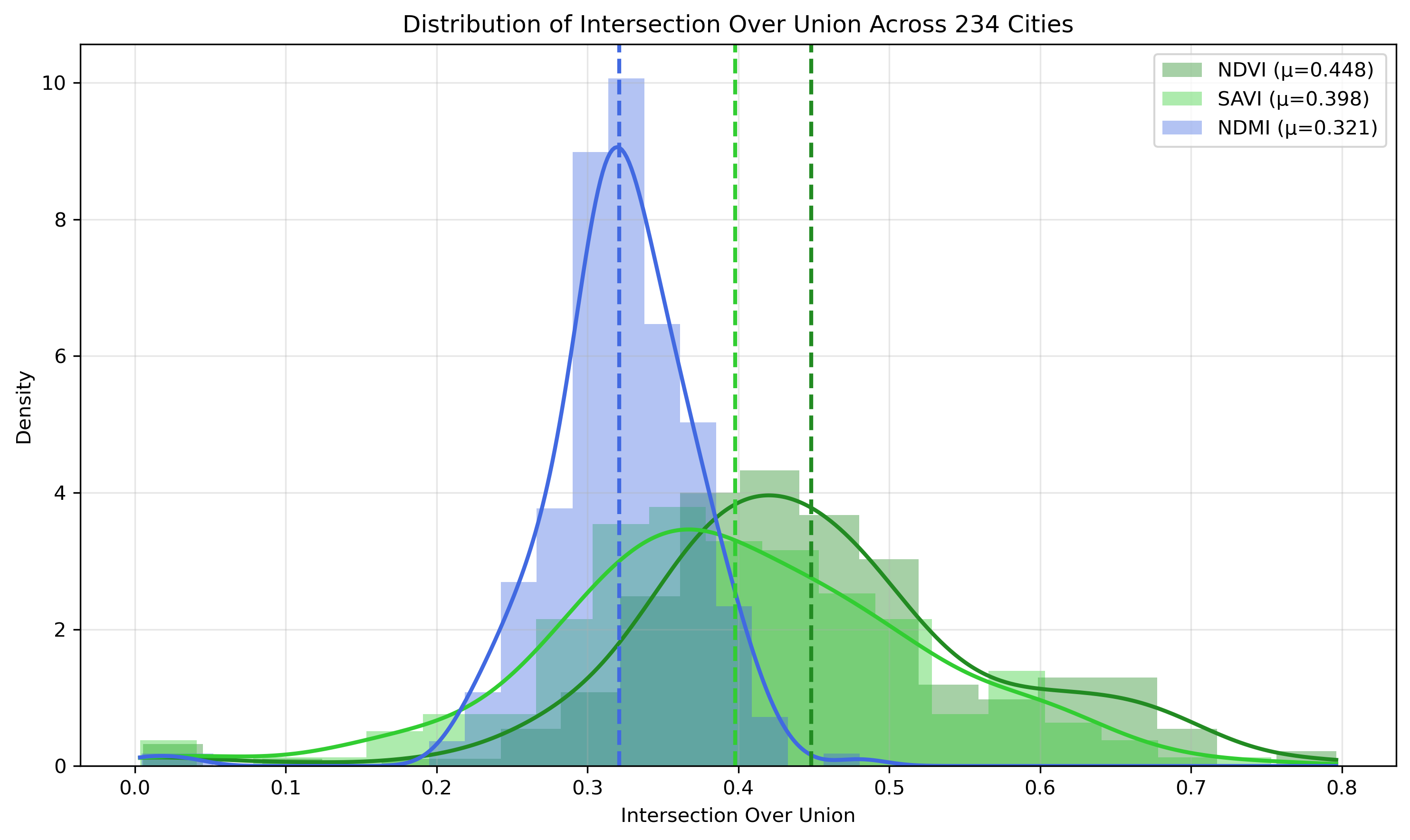
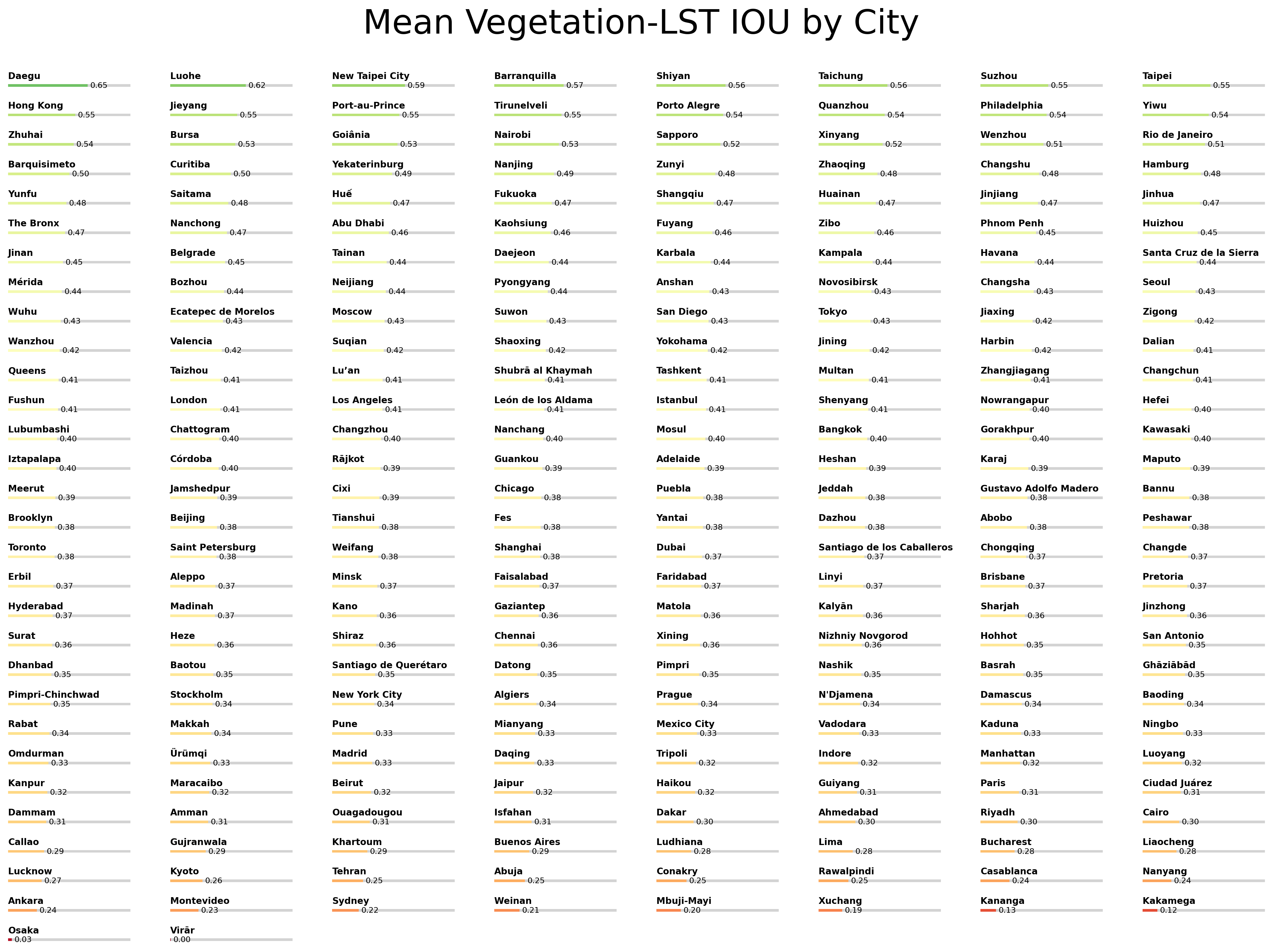
These masks were then evaluated for IOU with the results below:
Conclusion
As can be seen in the results above, there is clearly a correlation between a cities Land Surface Temperature and the presence of vegetation. This correlation, could be classified as moderate-strong when evaluated at a global level with varying levels of strength for different global region types.
Although the correlation is significant, it is clear that stronger correlations could be drawn if different approaches were taken. These improvements may include:
Improved LST Resolution – There is little to no high-resolution thermal data on a global scale available to the public. With improved LST resolution that matches current Sentinel2 observations, vegetation data may require less abstraction and therefore more direct correlations may be drawn between indexes. Besides hardware improvements, several attempts have already been made to improve resolution using thermal prediction models.
Direct vegetation segmentation models to replace vegetation indexes – The vegetation indexes in this report are generally regarded as strong indicators of vegetation presence and health when used at large scales. They are however, abstractions of two-band observations. Vegetation detection model have been shown to predict vegetation presence in a given pixel with high levels of accuracy using multi-spectral inputs. These bands could be used to make more precise measurements of vegetation presence on a much finer scale which may show stronger correlation to thermal indexes.
Altogether, this report was meant as a survey as several low-barrier methods to equate vegetation in urban environments to local temperatures. If you have any comments or suggestions for ways to improve this analysis I would welcome your feedback and would love to collaborate. Please reach out by clicking the “Lets Connect” button at the top or bottom of this page.
You can reference most of the code used in this analysis in the GitHub Repo here:
Use the "sample_workbook.ipynb" to follow along with the process to build the statistics used on this page