Synthetic Aperture Radar - Survey
A Survey of Synthetic Aperture Rader (SAR): with a focused use case on Ship Detection.
October 24th, 2026
Preface
Synthetic Aperture Radar (SAR) is an active radar technology that uses long-wave radar to detect objects on the Earth’s surface. Because SAR produces its own energy and because it uses long-wave radiation, it provides unique capabilities to observer the Earth’s surface in nearly all conditions – regardless of sunlight and cloud conditions. These unique attributes places SAR at the cutting edge of geospatial intelligence.
This report explores the basics of SAR data processing through a ship detection use case. Two methods were employed to investigate this use case: a deterministic image-processing model, which identifies bright clusters of pixels, and a fine-tuned deep learning model, which identifies a ship’s shape and backscatter signature. The purpose of this report is demonstrate baseline SAR data capabilities, while simultaneously building a basic repository of SAR data processing models. To support the latter, the codebase written for this report can be found at this GitHub Repo.
Two data sources were used for this report. First, Sentinel-1’s polarized backscatter data was collected through Planetary Computer to explore basic SAR products with their un-abstracted polarizations. Second, the SAR Ship Detection Dataset (SSDD) was employed for both ship detection models. The SSDD dataset provided SAR image tiles with accompanying ship labels in YOLO format. This set was useful model training and evaluation, however it did sacrifice some basic SAR information (polarization & phase data) for the sake of labels. A follow-up report might explore model performance on multi-channel SAR data.
Understanding the SAR Signal
Unlike optical imagery, where bright pixels generally represent strong reflection of sunlight within a particular spectral band (color), brightness in a SAR image represents the strength of the returned radar signal after the data have been processed for display. The strength of that return depends on several factors, including surface roughness, geometry, material properties, radar wavelength, and viewing angle. As a result, SAR signals do not have color, but rather amplitude (brightness), phase and polarization. These qualities return data that may be harder to understand by the human eye, but may provide more information about shape, and material than traditional EO/IR imagery.
Exploring Polarized Sentinel-1 Backscatter
To understand this data in action, this project used Microsoft's Planetary Computer STAC API to retrieve Sentinel-1 Radiometrically Terrain Corrected (RTC) data. A sample search covered an area of the western Mediterranean near southern Spain, with scenes collected during 2025. From STAC Items returned two polarization channels:
- VV — Vertically transmitted and vertically received radar energy.
- VH — Vertically transmitted and horizontally received radar energy.
I extracted a sample area from the georeferenced raster data and converted positive, linear backscatter values into decibels for visual comparison using 10 × log10(backscatter).
10 dB filtering is necessary for radar backscatter to diminish the signal to noise ratio and form an image. The result highlights how the same surface can appear differently
depending on the polarization used to observe it.
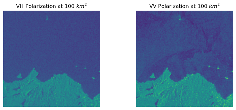
It is important to distinguish this product from raw or single-look complex (SLC) radar measurements. The RTC VV and VH assets here have had one layer of abstraction which means they do not account for phase data. This level of processing is appropriate for inspecting polarization-dependent intensity, but it is important that upstream data sources would be need to consider phase-sensitive analysis such as surface change.
Ship Detection Use Case
SAR Ship Detection Dataset (SSDD)
For vessel detection, the principal requirement was imagery paired with reliable ship-location annotations. This project used the SSDD dataset, retrieved from its Hugging Face dataset repository. The dataset contains processed SAR image chips and bounding-box labels identifying ships within each image.
Unlike the georeferenced Sentinel-1 RTC assets discussed above, these images were handled as conventional pixel arrays. This is an important distinction: the detection models in this report operate on the appearance of ships in processed SAR imagery, rather than directly on complex radar measurements or jointly on VV/VH polarizations. The decision to use this approach was data availability. As will be seen below, processed SAR images contain enough information for this use case, however, some edge cases may benefit from un-abstracted multi-channel SAR data.
The version of SSDD used in this analysis was already organized into training, validation, and test partitions. A simple data loader was built to inventory those partitions, associate images with their labels, validate the annotations, and convert the normalized YOLO bounding-box coordinates into pixel coordinates for evaluation. A basic breakdown of the SSDD dataset used in this exercise can be seen below:
| Dataset partition | Images | Annotated ships |
|---|---|---|
| Training | 789 | 1,756 |
| Validation | 139 | 285 |
| Test | 232 | 546 |
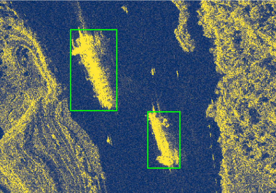
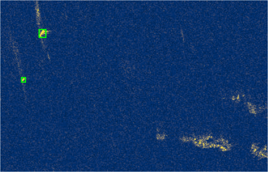
Below is an example of the data used in the detection experiments. The annotated bounding boxes provide the ground truth against which the models' predicted boxes can be compared. The first image shows two large ships passing through a small strait - note the high level of backscatter from the surrounding land. The second imagery captures two small craft at sea.
Methods
Two models were evaluated against the same 139 validation images, containing a total of 285 annotated ships. Keeping the evaluation data and matching procedure consistent made it possible to compare their strengths and weaknesses directly.
Evaluation Method
Each model returns bounding boxes describing the predicted location of a ship. To determine whether a prediction matches an annotated ship, I used Intersection over Union (IoU), which measures how much the predicted and reference boxes overlap relative to the total area covered by either box.
To be counted as a correct identification, an IoU of at least0.30 was required. This value was determined by trial and error. As will be seen below, the deterministic model naturally drew larger bounding boxes than the ground truth. The IoU was lowered to account for this since the primary goal of the use case was ship detection rather than accuracy. Eligible predictions and labels were then matched one-to-one, with an assignment procedure that favors the greatest number of valid matches and uses IoU to distinguish between alternatives. This prevented multiple predictions from receiving credit for the same annotated ship.
The results were classified as true positives (matched ships), false positives (unmatched predicted boxes), and false negatives (annotated ships without a match). From these counts, I calculated precision, recall, and F1 scores for individual images and aggregate summaries for the validation set.
The Deterministic Model
The first model intentionally used a simple assumption: in many open-ocean SAR images, a ship will be significantly brighter than the surrounding water. Instead of learning from labels, this detector applies an explicit sequence of image-processing rules.
For each grayscale image, the model calculates its mean brightness and standard deviation. It then marks pixels exceeding the following threshold:
Brightness threshold = image mean + 2 × image standard deviation
Pixels above the threshold are grouped into connected regions using eight-neighbor connectivity. Each region is assigned a bounding box, and the model retains candidates whose bounding boxes are at least 10 pixels wide and 10 pixels tall. The remaining boxes become the ship predictions.
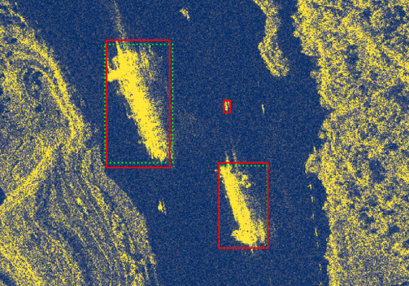
Below is a sample of the result of the three steps in this process:
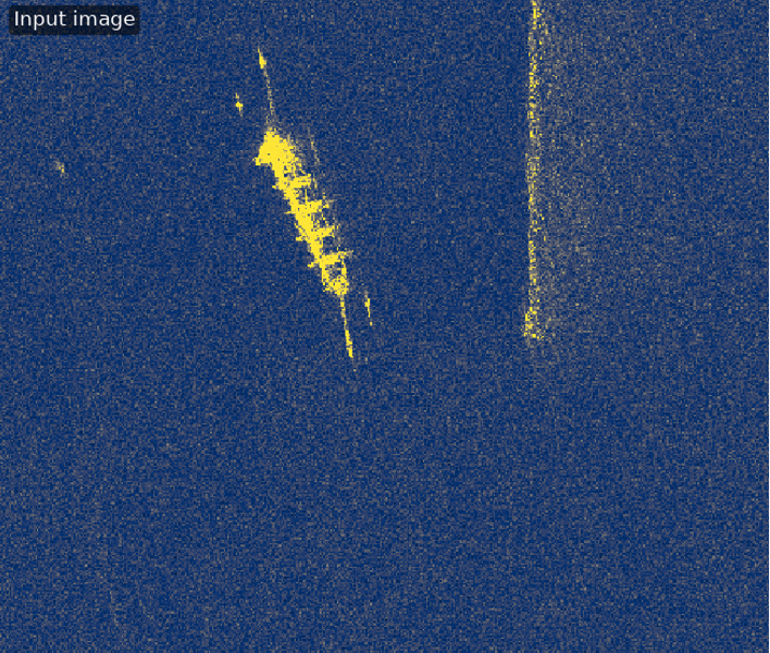
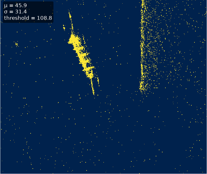
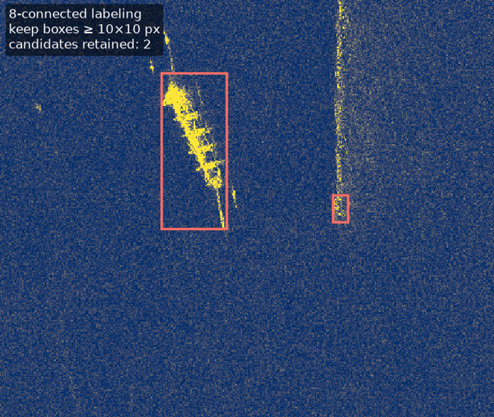
This method is computationally straightforward and easy to inspect. Each decision can be traced to a brightness threshold or a geometric filter, and those parameters can be changed to accommodate different kinds of imagery. However, the approach has an inherent limitation: a large bright region might be a vessel, but it could also be a shoreline feature, disturbed water, or another strong radar reflector.
Testing the model on one training image produced a successful match. Extending the analysis to the entire validation partition revealed a more complicated picture, especially for scenes containing coastal features and ship wakes.
The Deep Learning Model - YOLO v11
The second model used YOLO11n, a compact pretrained object-detection model. I began with pretrained yolo11n.pt weights and configured the model for a single
object class: ship.
The training configuration used the SSDD training and validation partitions, a 640-pixel input size, a batch size of four, and a target of 30 epochs with early stopping patience of ten. Training was conducted using PyTorch's Apple Metal Performance Shaders (MPS) backend. After the initial run was interrupted by a disk-space issue, the notebook includes a method to resume training from a saved checkpoint.
The available checkpoints were inventoried and compared before selecting one for evaluation. The final evaluation script loads the selected weights and runs inference on the same validation images used by the deterministic method, with the model's prediction confidence threshold set to 0.25.
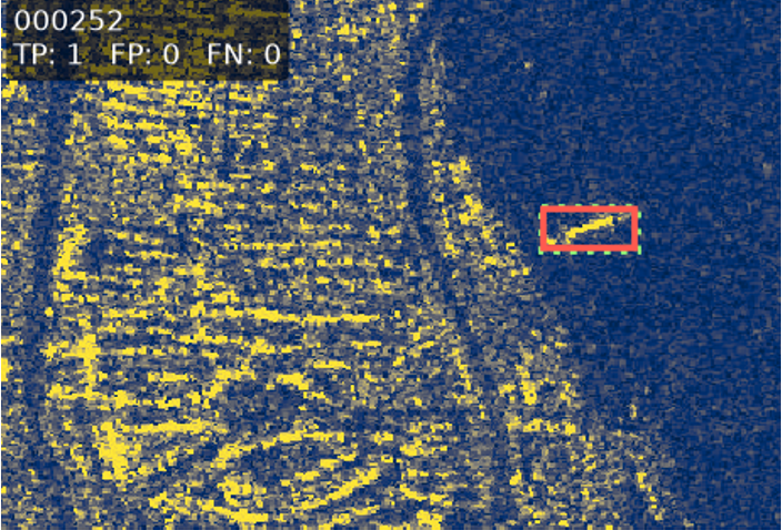
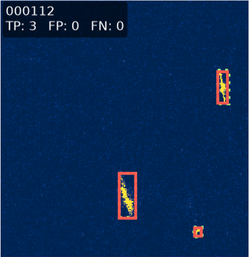
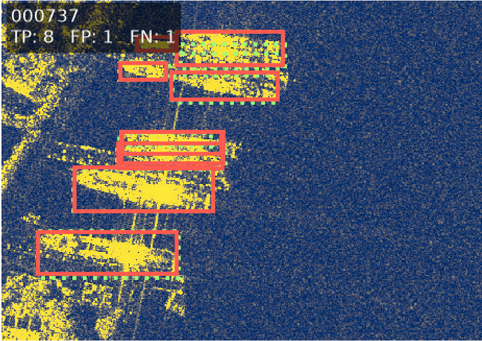
Where the deterministic detector relies on fixed pixel statistics, YOLO can learn visual patterns associated with annotated ships. This may include target shape, surrounding contrast, and context within the image. As a result, note how the Deel Learning model was able to better distinguish ships from other land-surface components.
Results
Validation Performance
The fine-tuned YOLO model outperformed the deterministic detector across the recorded validation metrics. Most notably, it matched 274 of the 285 annotated ships, compared with 217 using brightness thresholding. This increased overall ship recall from 76.1% to 96.1%.
| Validation metric | Deterministic | YOLO11n |
|---|---|---|
| Matched ships | 217 / 285 | 274 / 285 |
| Overall ship recall | 76.1% | 96.1% |
| Mean image precision | 58.6% | 94% |
| Mean image recall | 82.6% | 99% |
| Mean image F1 | 61.8% | 95% |
| False positives per labeled ship | 2.12 | 0.13 |
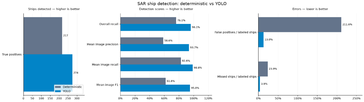
This contrast suggests that the visual information available in these SAR chips cannot be adequately described by image brightness alone. The learned detector was substantially better at distinguishing the ships' visual signatures from other bright areas in the same scenes.
Understanding Detection Errors
The aggregate scores tell only part of the story. Visual inspection of the predictions revealed two recurring challenges:
Shorelines and port environments. Coastal structures can generate high backscatter returns that interfere with the radar signatures of nearby vessels. The deterministic method is especially vulnerable because the scene's mean and standard deviation change as bright land features take up more of the image. YOLO is better able to distinguish many of these cases, but is not immune to clutter near land.
Ship wakes and disturbed water. Wakes can alter surface roughness and create bright or structured backscattering surfaces in radar imagery. A threshold-based detector may identify these features as separate objects, particularly when they form disconnected bright regions. The influence of surface-wave scattering provides a plausible physical explanation for some of these responses, although the imagery alone does not prove that any individual false positive was caused by Bragg resonance.
One useful example is validation image 000232. The deterministic detector produced many false-positive boxes and failed to match the annotated ships. On the same image, YOLO detected the annotated ship with no false positives under the project's IoU threshold.
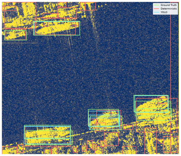
Other scenes show that learned detection is not perfect. For example, validation image 000036 produced one correct YOLO match but three false-positive predictions. These cases are useful reminders that the improvement seen in the overall scores does not remove the need for error analysis and domain-specific validation.
Conclusion
This project began as an exploration of SAR backscatter and developed into a comparison of two strategies for extracting useful information from processed radar imagery. Both models could detect ships, but their effectiveness differed considerably once they encountered the variation present across the validation dataset.
The deterministic method is valuable for its transparency, low complexity, and ease of customization. Its weaknesses arise from the assumptions built into its rules: unusually bright pixels are not always ships, and the brightness statistics of an entire scene can change dramatically near land.
The fine-tuned YOLO model performed substantially better, matching 96.1% of annotated ships on the validation images at IoU 0.30. Its results illustrate the advantage of learning visual patterns from examples rather than relying on a single intensity-based decision rule. That advantage must be weighed against the need for labeled training data, model maintenance, and testing on new acquisition conditions.
Several steps would strengthen this analysis in future work:
Sensitivity analysis. Varying the deterministic threshold and area constraints, YOLO's confidence threshold, and the evaluation IoU would reveal how much of the comparison depends on the chosen operating points.
Connecting detection back to richer SAR data. A future project could pair vessel-location labels with suitable Sentinel-1 acquisitions and examine how polarization, acquisition geometry, or complex-valued information affect detection. That would require a carefully constructed, temporally and spatially matched dataset; the present experiments do not establish those results.
More broadly, ship detection is only one stage of a practical maritime monitoring system. Useful operational information also depends on acquisition planning, geolocation, quality control, temporal association, and interpretation. This exercise provided an opportunity to understand the detection stage while remaining grounded in the physics and limitations of its underlying satellite observations.
The full code and exploratory notebook are available from my GitHub:
See main.ipynb for the step-by-step analysis, evaluation outputs, and selected detection examples.